Table 8. 2020 External O-D Table (1-hour PM peak vehicle trips)*
-----------------------------------------------------------------
 ORIG\DEST    1      2      3      4      5      6      7      8
-----------------------------------------------------------------
     1       10     25     25     25      0      0     50    100
     2       25     10     10     10      0      0     50    100
     3       25     10     10     50      0      0     50     50
     4       25     10     50     10      0      0    100    200
     5        0      0      0      0      0      0     50     50
     6        0      0      0      0      0      0    100    100
     7        0      0     50      0     50    100      0   1000
     8       50     50     50      0      0      0   1100      0
-----------------------------------------------------------------
 * For 1-hour PM peak hour (5-6 pm) (combined trip purposes)

5.2 User Equilibrium Assignment

Assign the base O-D matrix to the network via User Equilibrium Assignment (UE). This matrix now reflects internal vehicle trips generated, distributed, and factored in prior model steps, as well as IE, EI, and EE trips appended in Task 5.1, producing the full PM-peak hour (5-6 PM) vehicle trip O-D matrix. Report this final matrix.

5.2.1 Perform Trip Assignment
Determine the User Equilibrium (UE) solution using iterative trip assignment. The default method is the N-Conjugate Modification of the Frank-Wolfe (FW) algorithm, which starts with an initial All-or-Nothing (AON) Assignment using initial minimum path skim trees. The solution procedure iteratively applies: (a) link performance functions (to update link travel times), (b) a minimum path algorithm (to update network paths), and (c) an All-or-Nothing (A-o-N) Assignment (to compute a new assignment). A line search using the current AoN loadings and the prior assignment is used to determine the weight by which to combine these two sets of link flows into a new solution for the next iteration. While a variety of convergence indices can be applied, use Relative Gap (RG). The default RG is 0.01 but you should evaluate the results using a 0.001 RG value. Discuss the convergence process.

Assign the final PM-peak hour (5-6 PM) vehicle-trip O-D matrix to the base Miasma Beach highway network using User Equilibrium Assignment.

5.2.2 Evaluating the Assignment Results
Trip Assignment provides the flows (volume and travel time) for each direction of a link. A link's A-node and B-node must be identified to distinguish between AB_Flow and BA_Flow. This node information should be associated with each link in the Highways/Streets layer.

The tcw_rep.txt contains summary information on the assignment, including the Total VHT (Vehicle-Hours-Traveled) and Total VMT (Vehicle-Miles-Traveled) that are important performance measures for the Highways/Streets network. Save this file tcw_rep.txt to the work directory. In each required report, include these trip assignment outputs. Theme maps should also be created to graphically display network flows and to identify congested links.

5.2.3 Report the Assignment Results
Report and discuss the assignment results, including appropriate network maps, tables, and summary statistics.

1. Tabulate link volumes, resultant travel times, and volume/capacity (V/C) ratios
   [as always, sort by facility type]
2. Plot link volumes, resultant travel times, and V/C ratios
   [optionally, color-code V/C ratio ranges]
3. Tabulate network summary statistics (e.g., VMT, VHT, average speeds)
4. Discuss model convergence (relative gap, number of iterations, etc.)

5.3 Validation of Network Performance

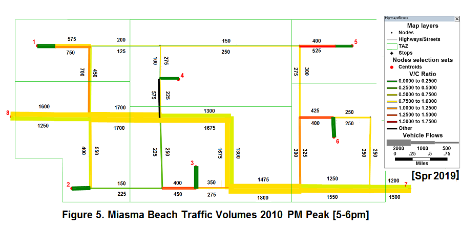
Compare your base assignment with the observed network flow pattern displayed in Figure 5 (volumes in vph). There are several levels at which model validation should be assessed:

1. System-level Measures
   System-level measures include outputs such as total vehicle miles traveled (VMT), total vehicle hours traveled (VHT), average travel time or average speed, etc. Travel time and speed results can be presented by link-types, mode-types, or even for selected O-D pairs. These measures begin to get at impacts on overall network delay (e.g., changes in travel time, changes in average speed, or estimated versus free flow travel times, on a link-type or network level). Also, summaries of total, interzonal, and intrazonal trips can be provided, by purpose, mode, and time-of-day.
   
   
2. Corridor-level Measures
   Screenlines provide a validation of overall travel in the study area. Application of screenlines in key corridor locations provides an assessment the ability of the model to replicate aggregate flows. Total observed flows across screen lines in both directions are compared with corresponding volumes estimated by the model system. It is still necessary to assess the overall performance of the network with system-level measures.
   
   
3. Link-level Measures
   These measure are developed for selected sets of links or link-types (e.g., all links in a specific area, all arterial links). Measure involve speed and travel time results, as well as volume capacity ratios. Theme maps can display links with travel times, speeds, or VC ratios over certain thresholds. Intersection turning movement can also be estimated (these estimates in turn can be used to assess intersection performance using Highway Capacity Manual techniques and/or software). Turning movement analysis may be done for selected intersections. These Link-level Measures are optional for Miasma Beach.

Include the following items in your validation analysis:

1. Report and compare system-level summary statistics for observed flows and the estimated model results.
   
   
2. Construct a minimum of three screen lines across which total flows are measured and compared. These screen lines, for example, might capture all flow across the network from east to west, or all flows into the downtown zones (1 and 2). Justify your choice of screen lines. Provide screen line summary maps and tables, clearly identifying the screen lines and the associated traffic volumes. Report deviations between observed and estimated volumes, by direction. Include goodness of fit measures.
   
   
3. Discuss the accuracy of the overall model system: Is the model system validated? Justify.